HOME Flying Quotes Paragliding Addictionary Whether to Fly DIY Electronics for PG Sites Logged Gallery A Diary Contact

Paragliding Weather

Motivation

As paragliding pilots, we need information about the weather that will help us in making judgments about the flying conditions.

For ridge soaring in dynamic lift conditions, we would like to know the wind direction and speed at launch.

For thermalling and flying XC, we would like to know the wind direction and speed at launch, the atmospheric instability and cloudbase height, and winds aloft.

In both situations, we would like to know if there are any wind shear layers, predicted storms, and how the conditions will change during the day.

Macro and Micro Weather Forecasts

At the macro level, the India Meteorological Department website provides wind and rainfall analysis and forecasts at a country scale of view.

At the micro level, the Global Forecast System (GFS) is a numerical weather forecasting model from the U.S. National Oceanic and Atmospheric Administration (NOAA) that provides weather predictions up to a resolution of 35km x 35km.

In order to provide accurate forecasts, the GFS model needs regular data from nearby weather stations. Specifically, it relies on radiosonde ‘soundings’.

A radiosonde is a helium filled balloon attached to telemetry instruments. The balloon is released and as it rises in the atmosphere, it relays data back to the weather station about the pressure, temperature, relative humidity, wind speed and direction, etc. Each sounding is effectively a vertical snapshot of the atmosphere at that location and time.

The NOAA and xcskies websites provide weather forecasts based on the GFS model. But before we can effectively use the information, we need to understand some concepts about pressure, altitude, temperature, humidity, and atmospheric stability.

The information in this article has been condensed from various online resources. I’ve tried to make the presentation concise. Please follow the links for more in-depth coverage of these topics.

The Basic Concepts

UTC / GMT / Zulu Time

Universal Time Coordinate, Greenwich Mean Time and Zulu Time all reference the same time origin. India is 5 1/2 hours ahead of UTC.

Pressure and Altitude

Atmospheric pressure is related to altitude. In the Troposphere (the layer closest to earth) the relationship can be modeled with the equation :

Z = (T_o / T_grad) * ( 1 - (P / P_o) ^ (T_grad * R / g))

where

Z is the altitude in metres above mean sea level

P is the pressure reading in Pascals

T_o = 288.15 Kelvin (15 Celsius)

T_grad = 0.0065 Kelvin / m

R = 287.052 Joules/Kelvin * kg

g = 9.80665 m/s/s

P_o is the pressure at mean sea level, nominally 101325 Pascals

This follows the 1976 US Standard Atmosphere model. Note that P_o is a nominal value and depends on the local weather conditions. On a stable day, P_o will be higher. On a stormy day, P_o will be lower.

From the equation, we can see that altitude is not proportional to pressure. Pressure changes more rapidly at lower altitudes.

QNH Altitude

This is the true altitude above mean sea level. To calculate QNH altitude we use the actual value of P_o if known, else we calibrate at a known altitude location by adjusting the value of P_o until the calculated altitude is correct.

QFE Altitude

This subtracts the true landing area altitude from the QNH altitude, so it is effectively altitude above the LZ.

Airspace Altitude/ Pressure Altitude/ Flight Altitude

This uses the nominal value of P_o = 101325 Pa. Airspace altitude is important for commercial aviation. All aircraft in a region read consistent airspace altitudes, even if they are incorrect. This allows them to maintain vertical separation.

Pressure Units : Bar / Pascals

1 bar = 100 kPa

1 mbar = 1 hPa = 100 Pa

Some weather prediction models show winds aloft for specific pressure values rather than altitudes. To guide you, here are some pressure-altitude equivalent values so you can check the conditions at your site altitude.

Dew Point

The dew point is the temperature to which a parcel of air must be cooled so that the moisture in the air condenses out.

The dew point is an absolute measure of the moisture in the air, independent of the temperature.

Relative humidity on the other hand, decreases as the temperature increases.

High dew points correlate well with what we perceive as oppressiveness or “mugginess”.

Temperatures during the night rarely fall below the evening dew point, because the latent heat of condensation offsets most of the cooling. This is why in coastal areas with high dew points, there is not much temperature difference between day and night, while in arid desert areas with low dew points, there is a large difference between day and night temperatures.

Temperature and Altitude

Temperatures generally decrease with altitude in the troposphere.

The Environmental Lapse Rate (ELR) is the change in temperature with altitude at a specific location and time. This is part of the data obtained from a radiosonde sounding.

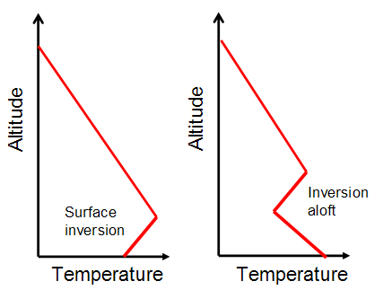
An ELR plot does not always show a steady decrease in temperature with altitude. There can often be inversion layers, where the temperature increases with altitude.

Adiabatic Lapse Rates

Air has low thermal conductivity. When a large homogeneous parcel of air moves in the atmosphere, there is very little heat exchange between it and the surrounding air. This is referred to as an adiabatic environment.

Consider a case where the parcel of air is not saturated with moisture (i.e., its temperature is greater than the dew point). The parcel may move up due to local triggers - terrain, convective, etc. As it moves up in the atmosphere, the pressure surrounding it decreases and the parcel expands. As it expands it cools, and this temperature lapse rate is called the Dry Adiabatic Lapse Rate (DALR). In the troposphere model, this lapse rate works out to approximately 10 Celsius / km.

When the parcel of air has risen and cooled to the dew point, the parcel is now saturated with moisture. As it rises and cools further, the moisture condenses out of the parcel of air, and releases the latent heat of condensation. As a result, the parcel of air no longer cools at 10 Celsius per km, but at a lower rate. For temperatures above freezing, the Saturated Adiabatic Lapse Rate (SALR) is approximately 5 Celsius / km.

Atmospheric Instability

Consider a parcel of air at the surface of the earth, whose temperature is well above the dew point at the surface, i.e. it is unsaturated. When this parcel moves up, it cools at the DALR of approximately 10 Celsius/km.

If the ELR is very low, a parcel of rising air will cool faster than the surrounding air, and therefore eventually lose buoyancy, and stop rising. In this case, the atmosphere is stable, and cloud formation due to convection is not possible.

If the ELR is very high, then the parcel of rising air will cool slower than the surrounding air, stay buoyant, and rise to its condensation level, forming cloud, and continue to rise - forming cumulus cloud. In this case we say the atmosphere is unstable.

A radiosonde sounding gives us the ELR and dew point at different altitudes. We can therefore estimate the atmospheric instability from this data.

Note that the atmosphere can have layers of stability and instability.

Estimating Cloudbase Altitude

As a first approximation, the dew point decreases with pressure (altitude) at a rate of about 2Celsius/km. The difference between the air parcel temperature and dew point temperature therefore decreases at a rate of about (10 - 2) = 8 Celsius/km.

If we know the temperature in Celsius of the parcel of air at the surface, and the dew point temperature in Celsius at the surface, we can estimate the altitude in km at which the parcel of air reaches dew point, by dividing the difference in temperatures by 8.

Example : If the actual surface temperature is 32 Celsius, and the dewpoint at the surface is 20 Celsius, the altitude at which the moisture will start condensing out of the rising air parcel is (32 - 20) / 8 = 1.5km above the surface.

Clouds in Stable Air

When the atmosphere is stable, clouds may be formed when air is forced upwards due to the topography, when it moves over a layer of colder air, or when two masses of air converge. The resulting clouds form horizontal layers or “Strata”.

Clouds in Unstable Air

When the atmosphere is unstable, clouds are formed by convective currents and eventual condensation. The saturated air in the clouds continues to rise until it is the same temperature as the surrounding air. The resulting clouds are vertically developed heaps or “Cumulus”.

Inversions and Thermalling

Morning surface inversions occur when the ground cools off rapidly during a clear-sky night.

Inversions aloft often happen when a warm air mass moves over a lower cold air mass.

Inversions are usually lower in a valley, and higher over ridges.

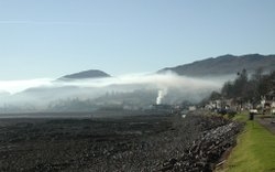
In dusty areas, inversions are marked by a grey or brown haze at the inversion layer.

In the picture below, you can see the smokestack spreading out horizontally at a surface inversion.

Most thermals will stop at an inversion layer. So on a day with weak thermals, inversions limit thermalling height gain. When thermalling, this feels like the paraglider bouncing off a “ceiling” - loss of cell pressure, slack lines, tip-collapses.

Strong thermals can “punch through” an inversion and continue to rise.

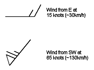
Wind Barbs

Wind on weather charts is visualized with icons called barbs that show both direction and speed. On the NOAA charts the speed is shown in knots - you can multiply by 2 (actually 1.8) to approximate the speed in km/hour.

A triangle = 50 knots

A full barb = 10 knots.
A half-barb = 5 knots

GFS Sounding Diagram

A GFS sounding is usually visualized as a Skew-T Log-P diagram. This has a grid of pressure and temperature lines on which the radiosonde sounding data is plotted.

The temperature grid lines on the X-axis are not vertical as in a normal graph, but tilted or ‘skewed’ to the right, to allow more data to be displayed in a portrait orientation page.

The pressure grid on the Y-axis uses a logarithmic scale, so that it is roughly linear in the equivalent altitude.

The rightmost irregular plot is the ELR plot, shown in red on GFS soundings from the NOAA. The DewPoint plot is by definition on the left, and is shown in green on GFS soundings from the NOAA.

Winds aloft are shown by wind barbs on a vertical scale corresponding to different atmospheric pressures - you can relate them to airspace altitude using the pressure-altitude table.

What the GFS sounding tells you about weather conditions

If the ELR and Dewpoint plots are far apart, you can expect cloudless skies.

If the ELR and Dewpoint plots are close together, you can expect thick cloud layers.

If the ELR plot kinks sharply to the right, you can expect an inversion layer at that altitude.

When the ELR and Dewpoint plots start far apart at the surface, and the ELR plot slopes rapidly towards the Dewpoint plot, you can expect atmospheric instability and cumulus cloud formation.

If the wind barbs show an abrupt change in wind direction, you can expect wind shear turbulence at that altitude.

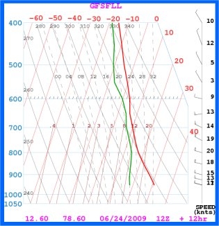
A Bad Weather Day at Bangalore

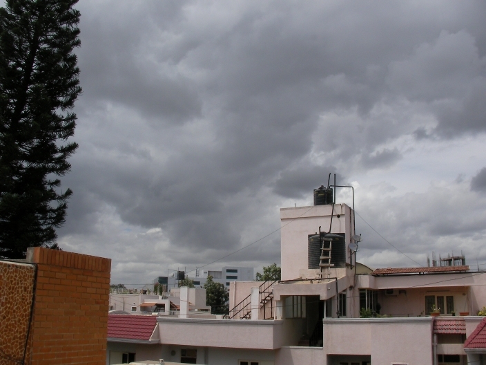
In the following GFS sounding the ELR and Dewpoint lines are close together. That is an indication of thick cloud.

Note also the abrupt change in wind direction at 700 mbar which indicates wind shear turbulence at the equivalent airspace altitude (~3000mASL).

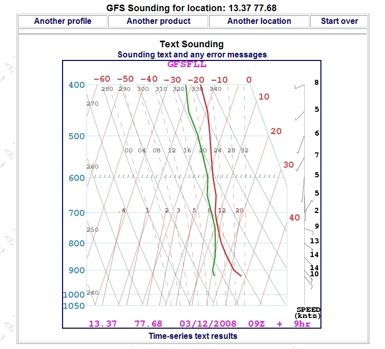
A photograph at Bangalore taken in the afternoon on the same day :

A Guide to the NOAA ARL website

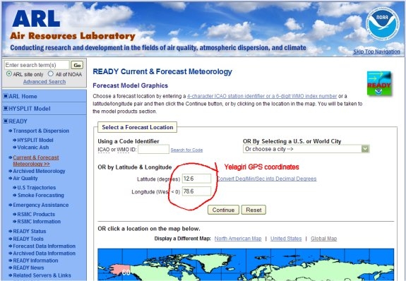
Click on the link to take you to the NOAA Air Resources Laboratory site. Enter the GPS coordinates of your site in decimal degrees (+ for East and North, - for West and South).

The site coordinates in this example are for Yelagiri, Tamil Nadu, India.

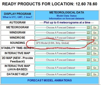
Click on Continue, then on the next page, select the Sounding Forecast using the GFS 84 hour, 3 hour interval option.

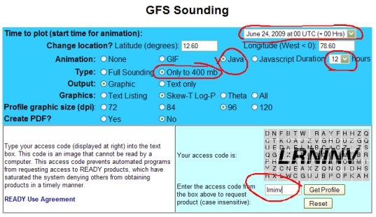
On the next page, select the start time for the forecast. Note that the times are UTC, so selecting 0 UTC is equivalent to 5:30am India Local Time.

Select the “Only to 400mb” option as this is the region of the atmosphere relevant to paragliding pilots flying without space suits.

Select the Java animation option with a 12 hour duration, as this will show you how the conditions change during the day from 5:30am to 5:30pm.

Finally, fill in the access code and click on “Get Profile”.

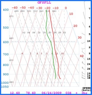
After the animation loads, you will see a repeating cycle of predicted Sounding plots. The example here is a forecast for Yelagiri on 24th June 2008, starting at 5:30am India Local Time and ending at 5:30pm, at 3 hour intervals.

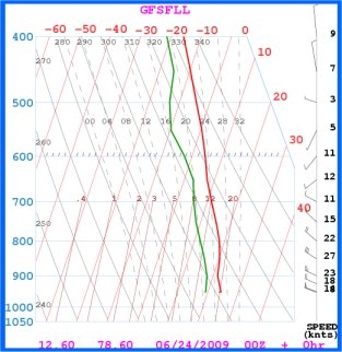
In the example shown here, you can see that the wind direction looks favourable for the west-facing sites at Yelagiri all through the day.

We can expect cloud cover through the day as the ELR and Dewpoint plots are close together.

Morning conditions do not appear to be favourable for paragliding, with high wind speeds of 30+ km/hour at the launch altitude of 1000m (~900 mbar).

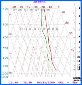
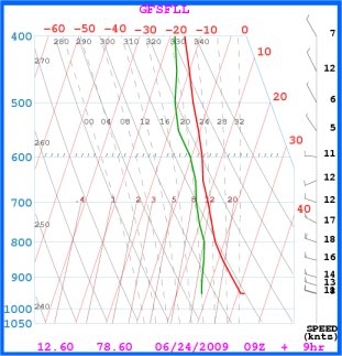
The conditions steadily improve during the day. Between 2:30pm and 5:30pm, thermalling may be possible due to the higher atmospheric instability and higher cloudbase (the ELR and Dewpoint plots starting farther apart).

Wind at launch has also dropped to about 25+ km/hour, but this is still strong, so the conditions look to be more favourable for dynamic ridge lift soaring at the western ridge face of Yelagiri.

We can estimate cloudbase at 2:30pm. At 1000m (launch height), the temperature from the ELR plot is about 27 Celsius At the same altitude, the Dewpoint is about 17Celsius. So cloudbase should be about (27-17)/8 = 1.25 km above launch.

A Caveat : Garbage In, Garbage Out

The GFS forecasting model accuracy depends on the presence of nearby weather stations providing frequent radiosonde sounding data. In Europe, this is not so much of an issue.

But closer to home, it’s a different story. For the Yelagiri site, the nearest weather stations providing daily radiosonde data are at Chennai, Hyderabad, and Bhubaneshwar !

Nevertheless, this is good knowledge to have. We don’t always fly at our home sites, and are now armed and dangerous with this slightly improved understanding of the weather.